

| • | Calculation |
| • | Base Conditions |
| • | Energy Conscious Solution |
| • | Example |
The CableApp uses the correction factors defined in the tables of Appendix 4 of BS7671. This allows the user to tailor a circuit rating for their given prescribed installation. These correction factors cover the following parameters: ambient temperature (air, and ground where appropriate), soil resistivity, depth, proximity of multiple circuits for ladder, tray, direct in ground and in ducts in the ground.
| Rating Factor Type | Correction Table Reference in BS7671 | Applicable Reference Method & Ratings Table(s) |
| Rating factors (Ca) for ambient air temperatures other than 30°CAmbient | Table 4B1 | Ref Method C, E & F Tables: All |
| Rating factors (Ca) for ambient ground temperatures other than 20°CAmbient | Table 4B2 | Ref Method D, Table 4E4A |
| Rating factors (Cs) for cable buried direct in the ground or in an underground conduit system for soil resistivitites (for Ref Method D) | Table 4B3 | Ref Method D, Table 4E4A |
| Rating Factors (Cd) for depths of laying other than 0.7m for direct buried cables and cables In buried ducts | Table 4B4 | Ref Method D, Table 4E4A |
| Rating factors for one circuit or one multicore cable or for a group of circuits of multicore cables, to be used with current-carrying capacities of Tables 4D1A to 4J4A | Table 4C1 | Ref Method A, B, C, E or F (appropriately) Tables 4D1A, 4D2A, 4D5; 4E1A, 4E3A & 4E4A |
| Rating factors for more than one circuit, cables buried directly in the ground (for Ref Method D, Table 4E4A) | Table 4C2 | Ref Method D, Table 4E4A |
| Rating factors for more than one circuit, cables in ducts buried directly in the ground (for Ref Method D, Table 4E4A) | Table 4C3 | Ref Method D, Table 4E4A |
| Rating Factors for groups of more than one multicore cable, to be applied to reference current-carrying capacities for multicore cables in free air (Ref Method E, for Tables 4D2A, 4D5 & 4E4A) | Table 4C4 | Ref Method E, Tables 4D2A, 4D5 & 4E4 |
| Rating Factors for groups of more than one single-core cable, to be applied to reference current-carrying capacities of single-core cables in free air (Ref Method F, for Tables 4D1A, 4E1A & 4E3A) | Table 4C5 | Ref Method F, Tables 4D1A, 4E1A & 4E3A |
Base Cable Installation Conditions for Cable Ratings
| Parameter | Condition |
| Ambient Air temperature | 30°C |
| Ambient Ground temperature | 20°C |
| Base installation depth (for cables installed in the ground) | 0.7m |
| Base soil resistivity (for cables installed in the ground) | 2.5 K.m/W |
This CableApp executes voltage drop calculations using the pre-defined values for voltage drop, published in Appendix 4 of BS7671 for the appropriate Cable Type Table.
| Cable Type | Current Rating Table Reference | Volt Drop Table Reference |
| Single-core 70°C thermoplastic insulated cables, non-armoured, with or without sheath | 4D1A | 4D1B |
| Multicore 70°C thermoplastic insulated and thermoplastic sheathed cables, non-armoured | 4D2A | 4D2B |
| 70°C thermoplastic insulated and sheath flat cable with protective conductor | 4D5 | 4D5 |
| Single-core 90°C thermoplastic insulated cables, non-armoured, with or without sheath | 4E1A | 4E1B |
| Single-core armoured 90°C thermosetting insulated cables (non-magnetic armour) | 4E3A | 4E4B |
| Multi-core armoured 90°C thermosetting insulated cables | 4E4A | 4E4B |
The following information provides guidance in energy efficiency, and the calculation method used to provide the Energy Conscious Solution in the CableApp.
The calculation requires the end user to define some of the parameters used in the calculation, within the "settings" menu of the CableApp.
The potential savings should be considered as guidance only.
According to Joules Law, whenever a conductor carry’s current, it will generate heat (thermal energy).
It can be demonstrated that the thermal energy of a cable corresponds to the following general expression:
Where:
| Ep | energy generated (lost on the line) [kWh] |
| n | number of loaded conductors (2 for single-phase/dc or 3 for three-phase) |
| c | number of cables per phase |
| R | conductor resistance [Ω / km] |
| L | cable length [km] |
| I | line current [A] |
| t | time [h] |
If the cross-sectional area (S) of a cable is increased, there will be a corresponding reduction in the resistance (R). When carrying the same current I, there will be a reduction in the energy lost (EP). This energy saving can be quantified both as a cost saving in electricity bills and a reduction in CO2 emissions.
The cable itself will be more expensive because it will have a higher cross-sectional area (S) but the installer will benefit from the following:
- Lower running costs, reduced energy bills.
- Reduced CO2 emissions, therefore an environmentally better proposition.
- Extended design life for the cable because it is operating at a lower temperature.
Standard design life is based on the cable being at its maximum load (maximum operating temperature) for every hour of that defined life in years.
- Improved short circuit capability - larger cross-sectional areas will carry higher currents in a fault condition.
- Potential to uprate the cable to carry higher loads in the future.
As a rule, cables do not carry the same current (I) continuously. For this reason, it is advisable to consider the mean square value of the current over time or at least to make an estimate.
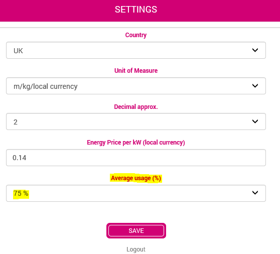
The CableApp will offer by default the average usage of load (I ') equal to 75% of I, but other values can be selected or defined by the user in the "Settings" of the CableApp
100% I
40% I (residential)
60% I (public place)
75% I (industrial)
Other %
Thus, the energy saved (EA) by installing conductors of lower resistance (R2) than (R1) will be:
Having calculated the saved energy, the economic savings can be calculated (£) and the savings in CO2 emissions since we have defined the electricity tariffs (Energy Price) in £/kWh (in the "settings") and the approximate values of CO2 emissions (ACO2) kg per kWh generated taking account of the country’s energy mix is defined by the CableApp. This value is set as a default within the CableApp and is taken from information published annually in the UK by the Department for Energy and Climate Change. Should you need to amend the default value, you can do so by selecting the “Advanced Calculation” option and updating the value provided in the CO2 Emissions Value field. It should be noted though, that once you have overridden this value, it will no longer automatically update each year when the government publishes the new value.
Care should be taken if using a value other than that published by the Department for Energy and Climate Change.
Applying the value for the electricity price and the value of CO2 emissions per kWh will therefore give the savings achieved by installing cross-section conductors with a larger section.
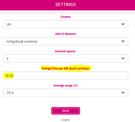
| Energy Price (tariff) | e.g. 0.14 £ / kWh | (this value is defined by the user in "Settings") |
| CO2 Emissions | e.g. 0.40 kg CO2 / kWh | (UK value published annually by UK government) |
Let’s assume we want to carry out an economic and ecological calculation as follows:
System - three-phase; 130 m; 268A
Cable Type - 6491X (Table 4D1)
App Proposed Technical Size - 95mm² copper conductor
To calculate the savings, we must consider increasing the cross-sectional area to a larger size.
The next largest standard cross-section to the 95mm² would be 120mm².
| Size | Resistance (Ω/km) | Size | Resistance (Ω/km) | |
| 1.5 | 14.478 | 120.0 | 0.183 | |
| 2.5 | 8.866 | 150.0 | 0.148 | |
| 4.0 | 5.516 | 185.0 | 0.119 | |
| 6.0 | 3.685 | 240.0 | 0.090 | |
| 10.0 | 2.190 | 300.0 | 0.072 | |
| 16.0 | 1.376 | 400.0 | 0.056 | |
| 25.0 | 0.870 | 500.0 | 0.044 | |
| 35.0 | 0.627 | 630.0 | 0.034 | |
| 50.0 | 0.463 | 800.0 | 0.026 | |
| 70.0 | 0.321 | 1000.0 | 0.021 | |
| 95.0 | 0.231 |
Reference is made in the background of the App to the electrical resistance table (above), calculated at a given average operating temperature. The R value for the next size is selected, in this case 120mm². For the simplicity of the calculation, both conductors are assumed to be operating at the same temperature. In reality, the resistance for the larger conductor will be lower than that given in the table when carrying the same load, because the larger conductor will be operating at a lower temperature. The subsequent savings will be a conservative estimate.
If the calculation is undertaken for an annual usage, then the time (t) will be 365d x 24h = 8760 h.
We will assume the average usage is 75% (default value in the App, but this can be changed in the “settings” menu)
Now you can calculate the energy that can be saved in a year using 120 mm² instead of 95 mm².
| EA | = (n/c x (R95 - R120) x L x (%U x I')² x t) / 1,000 |
| = (3/1 x (0.231 - 0.183) x 0.13 x (0.75 x 268) ² x 8760) / 1000 | |
| = 6625 kWh |
In the example, we have defined the chosen installation as a property with a tariff rate of £0.14 / kWh (remember the user should define their Tariff in the "settings").
In the example, the App has used a value for CO2 emission equal to 0.30 kg CO2 / kWh.
| Energy Price | 0.14 € / kWh | (This value is defined by the user in "settings") |
| CO2 emissions | 0.3 kg CO2 / kWh | (UK value published annually by UK government) |
| A£ | = 6625kWh x £ 0.14 / kWh = £927.54 | |
| ACO2 | = 4002 kWh x 0.3 kg CO2 / kWh = 1987.6 kg CO2 |
The calculated CO₂ saving, provided for the Energy Conscious Solution does not consider the increase in CO₂ emissions that are generated in manufacturing the larger cable size. The manufacturing CO₂ emissions will be small in comparison to the CO₂ saving for the circuit using the larger conductor size. This comparison will be even more pronounced over the lifetime of the cable.